GSoC 2026

NR Energy Modeling
for 5G-LENA Week 4

Standards Calibration (3GPP) + Real-Hardware Validation (SIGCOMM '21)

TR 38.864 (gNB) TR 38.840 (UE) GSoC 2026

Overview

What We Built

Added components:

NrGnbEnergyModel

TR 38.864 gNB power

NrUeEnergyModel

TR 38.840 UE power

NrUeDrxModel

C-DRX sleep/wake timers

NrPhyEnergyListener

Bridge to PHY traces

Energy = Σ state-power × time

gNB: symbol-level power accounting (14 sym/slot)
UE: state-based model with DRX occupancy
Two-track trust: match the standard and match real hardware

Architecture

Component Diagram

Data Flow

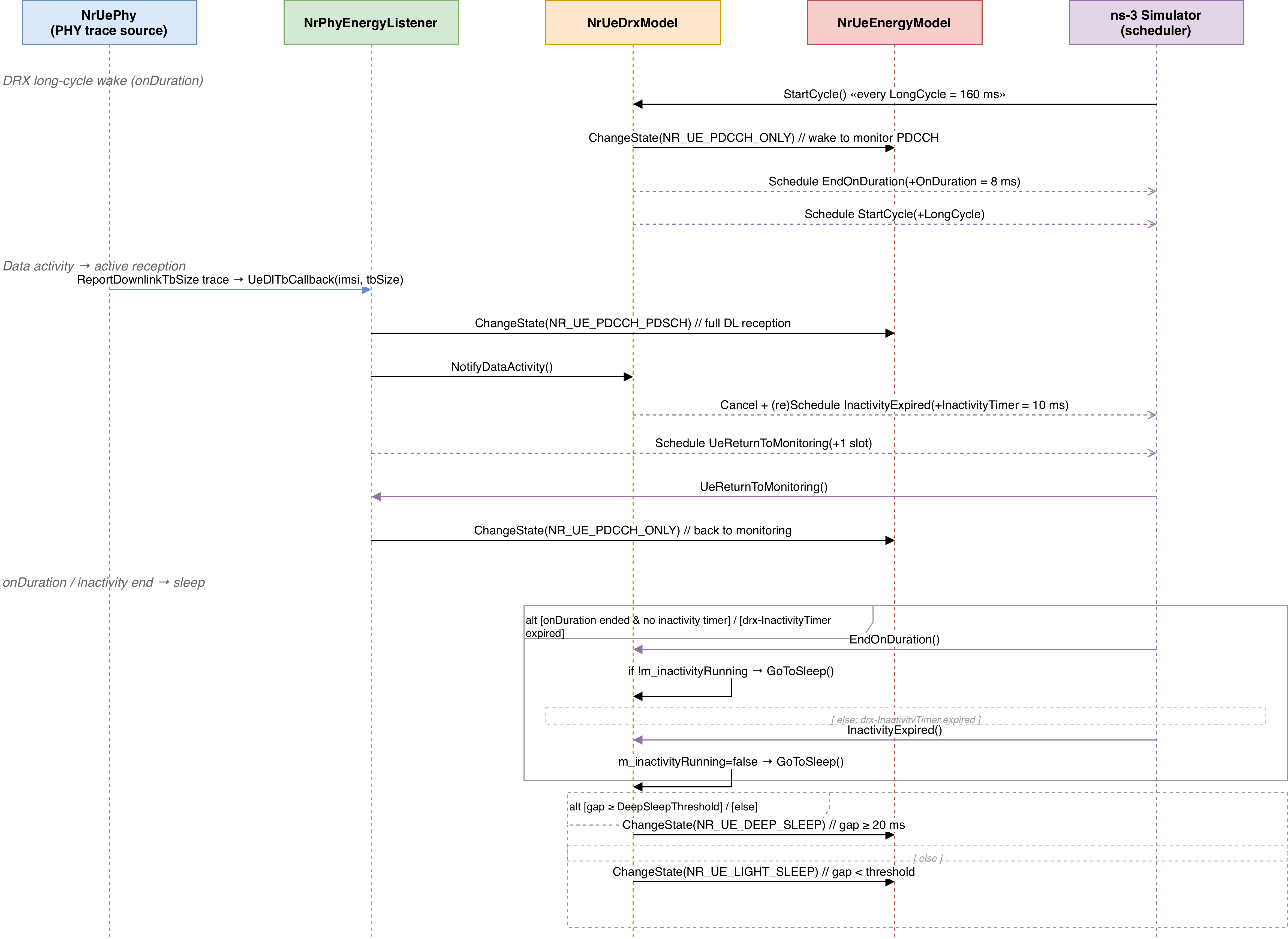
Per-Slot Event Pipeline

gNB PATH (PER SLOT)

1. NrGnbPhy emits "SlotDataStats" trace

2. NrPhyEnergyListener::GnbSlotCallback receives:

usedRegs, usedSymbols, availableRBs
→ sf = usedRegs / (availRBs × usedSymbols)
→ sp = txPower / refTxPower
→ sa = 1.0 (default, no antenna-muting data)

3. For each of 14 symbols in the slot:

DL sym → UpdateSymbolPower(DL, sf, sp, sa)
UL sym → UpdateSymbolPower(UL, sf, sp, sa)
F sym → UpdateSymbolPower(FLEX) = P3 (micro-sleep)

4. FinalizeSlotEnergy()

E_slot = Σ_sym P(sym) × T_sym → drains EnergySource

UE PATH (PER TB / DRX CYCLE)

1. NrUePhy emits "ReportDownlinkTbSize"

2. NrPhyEnergyListener::UeDlTbCallback:

throughput = tbSize × 8 / slotDuration
→ ChangeState(PDCCH_PDSCH)
→ SetActiveThroughputMbps(thr)
→ drx->NotifyDataActivity()
→ Schedule UeReturnToMonitoring(+1 slot)

3. UeReturnToMonitoring() fires:

ChangeState(PDCCH_ONLY)
SetActiveThroughputMbps(0)

4. NrUeDrxModel takes over:

InactivityTimer expires → GoToSleep()
gap ≥ 20 ms → DEEP_SLEEP
gap < threshold → LIGHT_SLEEP
Next LongCycle → wake to PDCCH_ONLY

Sequence Diagram

DRX Lifecycle: Wake → Active → Sleep

Verification Strategy

Two-Track Verification

01

3GPP Standards Calibration

Does the model reproduce the spec's own numbers?

TR 38.864TR 38.840

02

Real Hardware Validation

Does it reproduce Monsoon power measurements from real 5G devices?

SIGCOMM '21Monsoon

Track 1 — Standards

3GPP Calibration: gNB (TR 38.864)

Reference frame DDDSU, BS Cat1/Set1
Power parameters: P3=55, P4=280, P5=110 W
Closed-form full-load average over 70 symbols

P_DL = P3 + s_a(P4 − P3)[A + (s_f · s_p / η)(1 − A)]

234.714 W
Model output = Reference
0.000%
deviation (exact match)

Track 1 — Standards

3GPP Calibration: UE (TR 38.840)

Traffic: 3GPP FTP Model 1 (0.5 MB Poisson files)
C-DRX: 160/100/8 ms (long cycle / on-duration / inactivity timer)
Occupancy at λ≈10: 68% deep sleep / 28% PDCCH-only
3GPP ref: ~65% sleep / ~35% PDCCH-only

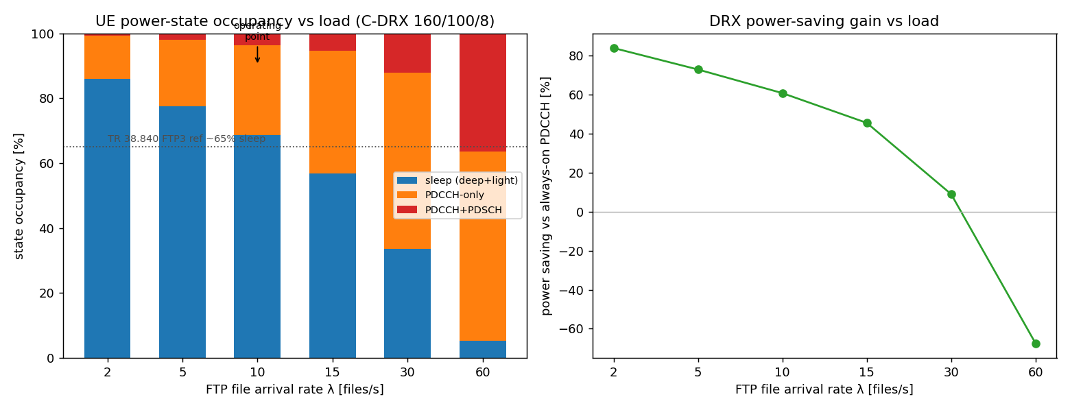
PDCCH+PDSCH gap: Our 28% PDCCH-only vs 3GPP's ~35% comes from the difference in how data arrivals reset the inactivity timer. Our model transitions back to PDCCH_ONLY after one slot, while the 3GPP reference assumes longer scheduler interaction — so we spend slightly less time monitoring and more time sleeping.

Why does power saving go negative? The right-side plot shows DRX savings vs “always-on PDCCH.” At very high λ, the UE is receiving data almost constantly anyway — DRX can't save anything because there are no idle gaps. The DRX overhead (wake-up transitions, on-duration monitoring) actually costs more than just staying awake, pushing savings slightly below zero.

Left plot: State occupancy fractions vs arrival rate λ. Deep sleep (green) dominates at low load, PDCCH-only (orange) grows with load. Right plot: DRX power-saving gain vs always-on — goes negative at high load when DRX overhead exceeds benefit.

Track 2 — Hardware Ground Truth

The Dataset: SIGCOMM '21

"A Variegated Look at 5G in the Wild" — researchers attached a Monsoon Power Monitor (a lab instrument that physically measures how many watts a phone draws over time) to Samsung 5G smartphones on Verizon's network in Ann Arbor, Michigan.

DATASET A — POWER-VS-LOAD (8805 rows, 1 Hz)

Each row = one second of a phone downloading data. Records the throughput the phone achieved and how much power the radio drew at that moment. We use this to check: “does our model predict the right power for a given load?”

Column	What It Means
downlink_Mbps	Measured 5G DL throughput (0–2442 Mbps)
hardware_power	Monsoon total − baseline = isolated radio power (mW)

DATASET B — RRC TAIL (~1.9M rows, 5 kHz)

A high-speed power trace (5000 samples/sec) that captures the phone's power over time as it connects, transfers data, and goes back to sleep. Just two columns: timestamp and power in watts. We use this to check: “does our model's power rise and fall at the right moments?” — specifically the RRC connection spike and the DRX tail duration.

AmmWave MI

Samsung phone on millimeter-wave (28 GHz) 5G in Michigan. 5127 1-second samples.

BmmWave MN

Different Samsung phone, also mmWave, in Minnesota. 17060 samples.

CLow-band MN

Same MN phone on sub-6 GHz (low-band) 5G. 5264 samples — lower throughput range.

Validation Framing

What “Validation” Means Here

We want to prove the model's power predictions match real measured power. The real measurements come from a Monsoon Power Monitor — a lab instrument that physically measures how many watts a phone draws over time.

THE ONE HONEST CATCH

The Monsoon only measured a phone (UE). Nobody put a power meter on an actual base station in this dataset. So we can't literally check “does the model's predicted tower watts equal real tower watts.” Instead we validate two things that can be checked, which is what A and B are.

✓

Can Check

Phone power vs load (A)
Phone power vs time (B)

✗

Cannot Check

Actual base station watts
(no gNB Monsoon data)

Validation A — “Power = Floor + Load × Traffic”

Plain idea: the busier a radio is, the more power it draws — and that relationship is a straight line (“affine”).

We feed real measured traffic levels into the C++ model and see if its predicted power tracks reality. R² = 0.495 = the best score any straight line could get on this noisy data — the remaining 50% is measurement noise, not a model flaw.

Why use the gNB formula? Because the UE model (TR 38.840) is flat during reception — it assumes the radio draws the same power whether receiving 10 or 1000 Mbps. A flat line has no slope, so you can't test “power grows with load” against it.

Proves: the power formula's shape is correct

Validation B — “Power Rises and Falls at the Right Times”

Plain idea: forget exact watts — does the phone's power rise and fall at the right moments?

We run the UE model through one connection cycle (idle → spike → ~9 s tail → idle) and overlay it on the Monsoon trace. Both curves are rescaled to 0–1 range (min-max normalised) because the Monsoon measures the whole phone while the model only predicts radio power. Direct UE-vs-UE comparison.

Proves: state structure + DRX tail timing

One-Line Summary

A Validates Shape, B Validates Timing

A: Shape of the Equation

Power = fixed baseline + (slope × traffic)
Checked using gNB model (the only one with a load slope).
Hardware: ~1.92 mW/Mbps × thr + 4500 mW.
Model matches this line.

B: Timing of Power States

idle → spike → connected tail (~9 s) → idle
Checked phone-vs-phone over a connection cycle.
Monsoon & model both show 3-level envelope.
Timing lines up.

Together: A validates the shape of the power equation, B validates the timing of power states — the two halves you'd need to trust the model, given there was no direct base-station measurement available.

Validation	Hardware Side	What It Proves	Comparison Type
A: gNB formula	UE radio power-vs-throughput	Affine load→power law + static fraction	Structural (law is right)
A-UE: UE model	UE radio power-vs-throughput	Same affine law, no gNB proxy caveat	Direct UE-vs-UE
B: UE + DRX	UE RRC power timeline	UE state structure + DRX tail timing	Direct UE-vs-UE
§9 slope ext.	UE power-vs-throughput	UE active-state slope (1.92 mW/Mbps)	Direct UE-vs-UE

Validation A — gNB load → power vs hardware

End-to-End Overlay: ns-3 Model vs Monsoon

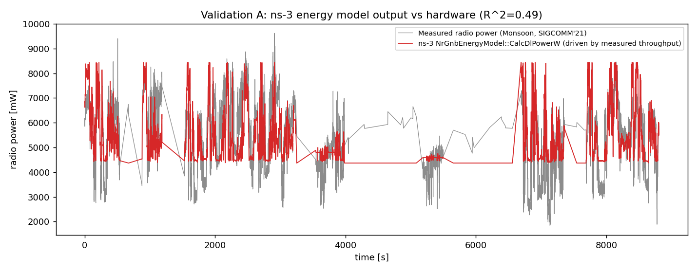
Insight: The model tracks every load spike and valley. R² 0.495 = the data's own OLS ceiling (0.499) — remaining 50% is real measurement noise (MCS/RSRP variation), not a model flaw. Issue: Only one scale parameter (PowerUnit = 30.1 mW) is fit; the shape comes entirely from 3GPP parameters.

HOW THE CSV WAS REPLAYED

The UE's measured throughput (from Dataset A) is fed row-by-row into the gNB model. Each row becomes one model prediction:

# Input CSV row (from Dataset A):
time=42.0, downlink_Mbps=850.3

# Model computation:
sf = 850.3 / 1900 = 0.4475
model_power = CalcDlPowerW(sa=1, sf=0.4475, sp=1)
= 145 + 135 × 0.4475 = 205.4 units

# Scale to mW:
predicted_mW = 205.4 × 30.1 = 6183 mW
# vs measured hardware_power = 6320 mW

This is done for every row. The 30.1 mW/unit scale factor is the only fitted parameter — found by least-squares: c = Σ(meas×unit) / Σ(unit²).

Validation A — Functional Form

Radio Power vs Throughput: Model vs Hardware

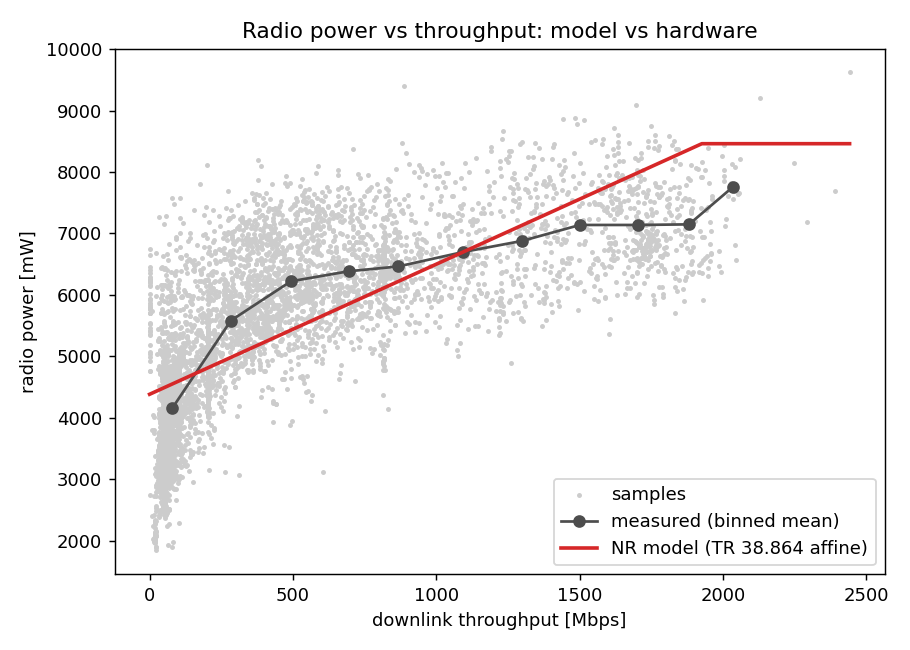
Hardware shows: static radio floor (~4.5 W) + load-proportional dynamic term — exactly the 3GPP form.

radio_power ≈ 1.92 mW/Mbps × thr + 4500 mW
(R² = 0.50, 5124 mmWave samples)

~2× dynamic range low to peak
Binned mean mildly saturating
R² 0.50 = noise floor (MCS/RSRP scatter)

Insight: The scatter plot confirms the 3GPP affine assumption holds in real hardware. Static floor at sf=0 is 145×30.1 ≈ 4365 mW vs hardware ~4500 mW (~3% gap). Issue: Saturation at very high throughput (>1800 Mbps) suggests a non-linear regime the linear model doesn't capture.

Validation A-UE — UE model driven by measured load

UE Model vs Monsoon: Direct UE-vs-UE

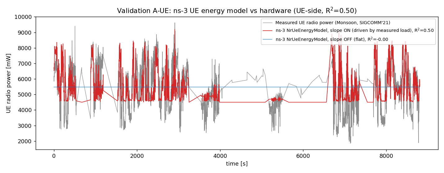
Red: UE model with slope ON (1.92 mW/Mbps) tracks the measured radio power. Blue dashed: flat TR 38.840 (slope OFF) — constant, cannot follow load. Grey: Monsoon hardware.

Why this matters: Validation A used the gNB formula as a proxy, which raised the question “but the data is from a phone, not a tower.” Validation A-UE removes that caveat entirely — here the NrUeEnergyModel itself is driven by the same measured throughput, and its power is overlaid on the measured UE radio power. Same device, same model, no proxy.

HOW IT WORKS

The UE is held in active reception (PDCCH_PDSCH) and emits:

model_mW = 300 + 1.92 × throughput
TR 38.840 active state (300 units) + ActivePowerSlope

We fit measured ≈ a·model + b, where b is the connected-idle RF floor.

Metric	Value
R² (slope ON)	0.499
NRMSE	18.5%
Dynamic gain a	1.000 — no rescaling needed
Fitted floor b	4199 mW (≈ hardware ~4.5 W)
R² (slope OFF)	−0.00 (flat = useless)
Static frac (floor:peak)	model 0.55 vs measured 0.51 (~8%)

Strongest result: the dynamic gain a = 1.000 means the 1.92 mW/Mbps slope calibrated on the MI dataset is the right absolute slope for this hardware — not just the right shape. Turning slope off collapses R² to 0.

Validation B — UE DRX tail vs hardware

UE Model: RRC Tail Envelope

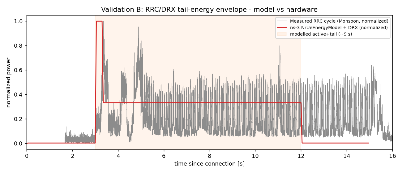
Y-axis is normalised 0–1 (min-max scaling). Both curves are rescaled so their minimum = 0 and maximum = 1. This is necessary because the Monsoon measures whole-phone power (1.70–7.46 W) while the model only predicts relative radio power (0.05–0.27 W) — absolute watts differ, but the shape and timing can be compared.

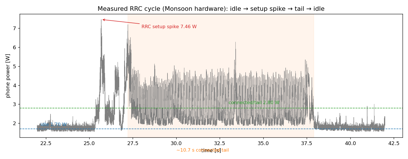
What was fed to the simulation: Nothing from Dataset B is fed into the model. Dataset B is only the ground truth to compare against. The model runs autonomously: we schedule one data burst at t=3 s, then let NrUeDrxModel’s timers (160/100/8 ms) handle the rest. Power is sampled every 50 ms via ΔE/Δt from GetTotalEnergyJ(). The resulting curve is then overlaid on the Monsoon trace.

Measured Monsoon: idle 1.70 W → spike 7.46 W → tail 2.80 W. ~10.7 s tail.

Why this matters for modeling: The tail duration (~9–10 s) is controlled by the DRX inactivity timer — matching it confirms our timer implementation is correct. The spike:tail power ratio (2.66×) tells us the SetupTransitionPower value for this device. To fit watts to UE hardware: measure the Monsoon idle-vs-active delta, set PowerUnit = (measured active − measured idle) / (model active − model idle). For this phone: PowerUnit ≈ (2.80 − 1.70) / (0.10 − 0.05) = 22 mW per model unit.

Gap #1 — The 3GPP Limitation

Flat State vs Hardware Reality

THE 3GPP LIMITATION

TR 38.840 assumes a flat energy cost for active reception, regardless of whether the UE is downloading at 10 Mbps or 1,000 Mbps. The standard gives one power number for the entire PDCCH+PDSCH state.

THE HARDWARE REALITY (SIGCOMM '21)

Empirical data from Samsung 5G smartphones proves active power scales linearly with data load:

Radio Power ≈ Slope × Throughput + Static Base

MEASURED SLOPES BY BAND & DEVICE

mmWave (MI)

1.92

mW/Mbps

mmWave (MN)

1.03

mW/Mbps

Low-Band

0.76

mW/Mbps (flatter)

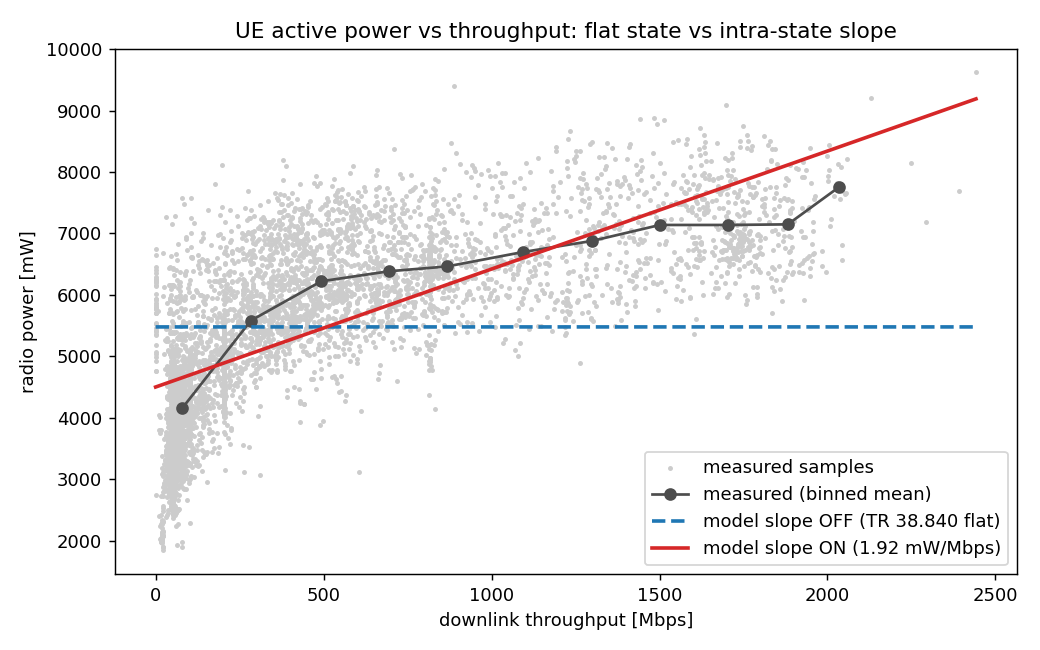
Blue dashed: TR 38.840 flat (R²≈0). Red: slope ON (1.92 mW/Mbps). Grey: Monsoon.

Insight: The flat blue line (3GPP default) explains 0% of throughput variance. Adding a simple linear slope captures the hardware trend. Issue: The slope varies by band and device (1.92 for mmWave MI, 0.76 for low-band) — no universal constant exists, so it must be set per scenario.

Implementation & Validation

ActivePowerSlope in ns-3

IMPLEMENTATION (model/nr-ue-energy-model.*)

In GetStatePowerW(), PDCCH+PDSCH becomes:
P = P_state·PowerUnit + ActivePowerSlope × throughput

New attribute: ActivePowerSlope [mW/Mbps], default 0.0 (= pure 3GPP)
New input: SetActiveThroughputMbps(mbps)
Bridge: UeDlTbCallback → throughput = tbSize×8/slotDuration
UeReturnToMonitoring() resets to 0
Default-off → 3GPP calibration unchanged

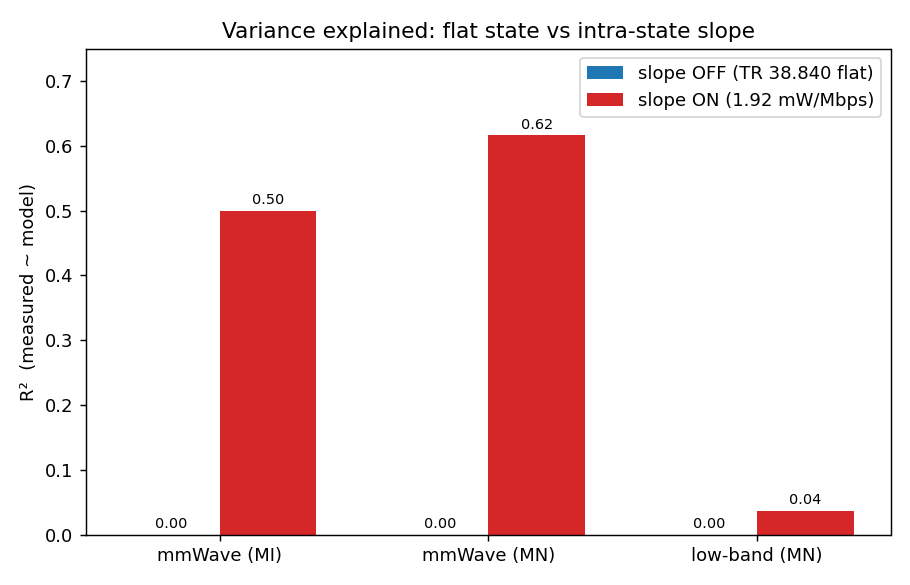
X-axis: dataset (mmWave MI, mmWave MN, low-band MN). Y-axis: R² (variance explained, 0–1). Blue = slope OFF, red = slope ON.

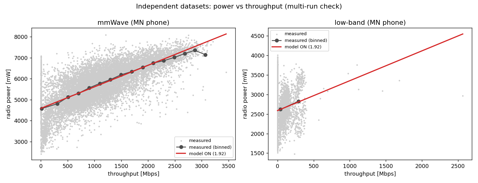
Insight: R² jumps from ~0 to 0.50–0.62 on mmWave when the slope is enabled. Low-band gains little (0.04) because its radio power barely depends on throughput. Issue: The extension is purely data-driven and not in any 3GPP spec — it's an empirical correction.

Independent runs on MN mmWave (left) and MN low-band (right). Low-band power barely depends on throughput.

Dataset	n	Slope	ON R²
mmWave MI	5127	1.92	0.50
mmWave MN	17060	1.03	0.62
low-band MN	5264	0.76	0.04

5-FOLD (MI): 2.11 ± 0.60 mW/Mbps, R² 0.55±0.06

Slope is band/device-dependent → exposed as a per-scenario attribute, not a constant.

Gap #2 — Transition Transient

RRC Connection-Setup Spike

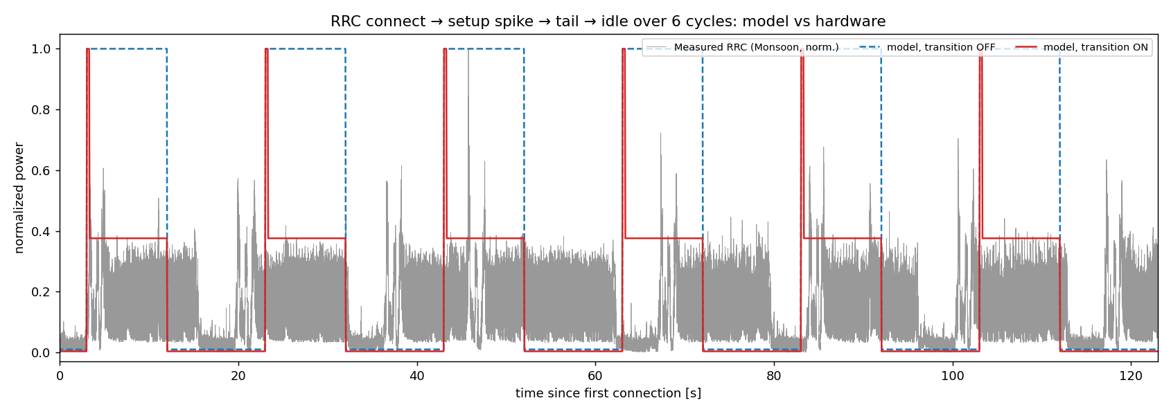
Six connect→spike→tail→idle cycles. Red: transition ON. Blue dashed: OFF. Grey: Monsoon.

Why it doesn't look like an exact match: The model's spikes are sharp rectangles (instant state change), while the hardware's are rounded (analog ramp-up of real circuitry). Also, the model's y-axis is in relative units (~0.05–0.27 W) while hardware is absolute (~1.70–7.46 W). What matches is the ratio (spike:tail = 2.66× in both) and the timing of each cycle, not the pixel-level overlay.

WHAT WAS FED INTO THE SIMULATION

Nothing from Dataset B was fed in. The simulation runs autonomously: 6 data bursts are scheduled at regular intervals. Each burst triggers:

# UE in DEEP_SLEEP, TB arrives:
TriggerSetupTransition(0.166, 300ms)
→ power jumps +0.166 W for 300 ms
ChangeState(PDCCH_PDSCH)
→ active reception for data duration
# Data ends, inactivity timer starts:
ChangeState(PDCCH_ONLY) ← tail
# After 8 s inactivity:
DRX → GoToSleep() → DEEP_SLEEP

Dataset B's Monsoon trace is only the ground truth we compare against, not an input to the model.

	Peak	Spike:Tail
OFF	0.100 W	1.0×
ON	0.266 W	2.66×
Hardware	7.46 W	2.66×

Methodology

How Data Was Fed Into the Code

REPLAY PATH — VALIDATION A (gNB)

CSV row

→

sf = clamp(thr/1900, 0, 1)

→

CalcDlPowerW(1, sf, 1)

→

replayA.csv

→

overlay_ab.py

No Simulator::Run — pure replay through C++ model. model_unit = 145 + 135·sf. Scale fit: c = Σ(meas·unit)/Σ(unit²).

DRX TIMELINE — VALIDATION B (UE)

t=0 DEEP_SLEEP

→

t=3 PDCCH_PDSCH + NotifyDataActivity

→

t=3.3 PDCCH_ONLY (tail)

→

t=12 InactivityTimer → DEEP_SLEEP

Power sampled every 50 ms: power = ΔE/Δt from GetTotalEnergyJ(). Runs on ns-3 Simulator timeline.

LIVE PATH — REAL SIMULATION

gNB SlotDataStats trace

→

sf = usedReg/(availRb×usedSym)

→

NrGnbEnergyModel

UE ReportDl/UlTbSize trace

→

ChangeState + SetActiveThroughputMbps

→

NrUeEnergyModel

No PHY edits — existing traces

TRAFFIC

FTP Model 1 (calibration) / UDP (throughput gen); energy drained from standard ns-3 BasicEnergySource.

Configuration

Simulation Setup

Platform

ns-3.47 + nr module
GridScenario: 1 gNB + 4 UEs

PHY

FR1 @ 3.5 GHz, 100 MHz, numerology 1 (30 kHz SCS)
TDD: DL|DL|DL|S|UL (DDDSU), 43 dBm, UMi

Energy

BasicEnergySource per node
NrGnbEnergyModel Cat1/Set1 (P3=55, P4=280, P5=110, A=0.4)
NrUeEnergyModel FR1
NrUeDrxModel 160/100/8 ms
Wired by NrPhyEnergyListener

Harnesses

cttc-nr-energy-calibration (3GPP track)
cttc-nr-energy-replay:
• --mode=replay (Val A)
• --mode=uereplay (Val A-UE + slope)
• --mode=rrctail (Val B)

Summary

Results Summary

	Check	Result
✓	gNB DDDSU (TR 38.864)	model = ref, 0.000%
✓	UE occupancy (TR 38.840)	68/28% vs ~65/35% (3GPP ref)
✓	gNB vs hardware (Val A)	R² 0.495 (≈ empirical 0.499), static frac 0.52 vs 0.55
✓	UE vs hardware (Val A-UE)	R² 0.499, dynamic gain a = 1.000 (no rescaling)
✓	UE DRX tail (Val B)	3-level envelope + ~9 s tail reproduced
✓	UE slope vs hardware	OFF 0 → ON 0.50–0.62 (mmWave)
✓	Transition spike	model 2.66× = measured 2.66×

Conclusion

Can We Go Ahead With This Modeling?

Yes.

Standards-exact where the spec is closed-form (gNB: 0.000%)
Regime-accurate and load-monotonic for UE (DRX occupancy within 3%)
Hardware-tracking to the noise floor (R² 0.495 = empirical ceiling)
Data-driven extensions capture real-world slope + transition spike

Honest Scope

UE slope is band/device-dependent → attribute, not constant
Setup-spike magnitude is empirical (not in TR 38.840)
One absolute scale (PowerUnit) fit per scenario
Val A feeds measured throughput, not sim-generated

Next Steps

Condition the slope on SINR (dataset has nr_ssSinr)
Wire transition energy from TR tables
Full-sim throughput generation for Val A

NR Energy Modelingfor 5G-LENA Week 4